STIS currently supports four basic operating modes:
ACCUM operating modes for the CCD and MAMAs, which produce a time- integrated accumulated image. These are the most commonly used modes.
TIME-TAG operating mode for the MAMA detectors, which outputs an event stream of high-time-resolution observations in the UV.
ACQ (acquisition) and ACQ/PEAKUP operating modes for the CCD and MAMAs used to acquire targets in the spectroscopic slits and behind coronagraphic bars and masks. Target acquisitions are described further in Chapter 8.
The STIS CCD has only the single operating mode, ACCUM, for science data. The CCD pixels accumulate charge during the exposure in response to photons. The charge is read out at the end of the exposure at a selectable gain (number of electrons per DN) and converted to 16 bit data numbers (DN) by the A-to-D converter. The DN are stored as 16 bit words (with a range 0 to 65,535) in the STIS data-buffer memory array. At the default CCDGAIN=1, the gain amplifier saturation level (33,000 e-), and not the 16-bit format, limits the total counts that can be sustained in a single exposure without saturating (see also Section 7.1.10 and Section 7.2.1). At the other supported gain, CCDGAIN=4, the CCD full well (144,000 e- or 36,000 DN, except in the outermost regions of the CCD where the full well is 120,000 e-, see Chapter 7 for details) still determines the saturation limit.
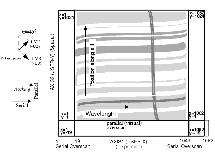
A full detector readout is actually 1062 x 1044 pixels with physical and virtual overscans. Scientific data are obtained on 1024 x 1024 pixels, each projecting to ~0.05 x 0.05 arcsecond on the sky. The dispersion axis runs along axis1 (image x or along a row of the CCD), and the spatial dimension of the slit runs along axis2 (image y or along a column of the CCD). Figure 11.1: illustrates the full CCD format and its orientation with respect to the spacecraft (U2 and U3 or V2 and V3) axes. Arrows indicate the orientation of the parallel and serial clocking. The readout directions depend on the amplifier used. For the default amplifier D, the readout is at the upper right corner. It includes 19 columns of leading and 19 columns of trailing physical overscan in axis1, and 20 trailing rows of virtual overscan in axis2. The trailing serial overscan as well as the parallel overscan pixels are used to determine the bias level in post-observation data processing. The parallel overscan can also be used in the diagnosis of charge-transfer problems.
The minimum CCD exposure time is 0.1 second and the maximum possible exposure time is 4.7 hours (though we cannot imagine wanting a single exposure longer than 60 minutes). The minimum time between identical exposures for CCD full-frame (1062x1044) images is ~45 seconds.1 This time is dominated by the time it takes to read out the CCD (29 seconds for the full frame) and can be reduced to ~19 seconds if you use a subarray (see CCD Subarrays).
The CCD supports on-chip binning. When on-chip binning is used the specified number of pixels in the serial and parallel directions is read out as a single pixel. The advantage of CCD binning is that the read noise per binned pixel is comparable to the read noise per unbinned pixel. Thus if your signal-to-noise per pixel is dominated by read noise when no binning is used, you can increase the signal-to-noise by binning. The disadvantages of using on-chip binning are (a) that it reduces the resolution of your spectrogram or image, (b) that the relative number of pixels affected by cosmic rays increases, and (c) that the relative number of 'hot' pixels (which is ~1% of all CCD pixels for unbinned data by the time this handbook is issued, see Chapter 7), increases by a factor proportional to the binning factor. On-chip binning of 1, 2, or 4 pixels in both the AXIS1 and AXIS2 directions is supported. Note that on-chip binning is not allowed when subarrays are used.
The number of hot pixels has been increasing steadily with time due to accumulated radiation damage on the STIS CCD (see the discussion on hot pixels in Chapter 7). Thus the impact of hot pixels on binned data has become significantly larger. Also note that when spectral data are spatially rectified, a single pixel in the original data will be interpolated into four pixels in the rectified image. For data binned NxM on board the spacecraft, a single bad pixel will, after rectification, affect the equivalent of 4xNxM pixels in an unbinned image.
When using the ETC to estimate the effects of on-board binning on the S/N of CCD observations, be aware that increasing the binning in the dispersion direction may cause the ETC to use a larger resolution element for its S/N calculation. Be sure to understand how much of any increase in the S/N number output by the ETC is due to an actual decrease in the read noise and how much is simply due to a change in the size of the resolution element assumed for the calculation.
During Phase 2, you specify the binning for your CCD observations using the BINAXIS1 and BINAXIS2 optional parameters. The default values are 1.
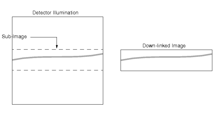
Subarrays can be used when the CCD detector is read out. Generally, there is no need to use a subarray for STIS data. The main scientific use of CCD subarrays is for time-resolved optical spectroscopy, where subarrays can be used to reduce the CCD read time and keep the data volume at a manageable level. CCD subarrays can also be specified for CCD acq/peak observations to limit the region in a diffuse object (e.g., a galaxy) over which the flux is summed for the peakup. When a subarray is used, only the portion of the detector which is within the specified subarray is read out and transmitted to the ground (see Figure 11.2-note that the spectrogram curvature is exaggerated in this figure).
As described in Section 11.1.1, full-frame CCD readouts are composed of 1062 x 1044 pixels: 1024 x 1024 data pixels, 19 leading and 19 trailing serial-overscan pixels, and 20 trailing parallel-overscan pixels. Dispersion runs along axis1 and the long dimension of the slit runs along axis2. Subarrays are required to span the full width of the CCD detector in the serial (dispersion) direction in order to ensure they contain the serial overscan needed to determine the bias level; however, you can control the height of the subarray in the parallel direction (i.e., along the slit for long-slit spectroscopic observations). Note that no parallel overscan is returned for subarrays (see also Section 7.2.5). Subarray size is specified in Phase 2 by the parameter:
The minimum allowed value of SIZEAXIS2 for ACCUM mode observations is 30 pixels (corresponding to 1.6 arcsec), and SIZEAXIS2 must be an even number of pixels. By default the target is placed within a few pixels of the center of the subarray. For a few central wavelength settings, however, the target may be systematically offset by up to 30 pixels in the spatial direction. Observers should consult with help@stsci.edu prior to using SIZEAXIS2 with a value of less than 64 pixels.
Use of Subarrays to Reduce the CCD Read Time
The minimum time between identical CCD exposures is the readtime + 16 seconds. The time to read out a CCD subarray is:

Thus, using the smallest available subarray, which is 30 pixels high, you can reduce the minimum time between identical exposures to ~19 seconds (16 seconds overhead plus 3 seconds read time). The minimum time between full-frame CCD exposures is 16 + 29 = 45 seconds.
Use of Subarrays to Reduce Data Volume
The format of the data you receive when you use a CCD subarray will have dimensions 1062 x sizeAXIS2, will cover the full range in the dispersion direction, and will include the serial overscan. The STIS buffer can hold eight full-frame CCD exposures at one time, or 8 × (1024 / sizeAXIS2) exposures at any one time. Full-frame CCD data acquired in one exposure can be transferred to the HST data recorder during the subsequent exposure(s) so long as the integration time of the subsequent exposure is longer than 3.0 minutes. If you are taking a series of exposures which are shorter than that, the buffer cannot be emptied during exposure, and once the STIS buffer fills up, there will be a pause in the exposures sequence of roughly 3 minutes as the buffer is emptied. This problem can sometimes be avoided with the judicious use of subarrays.
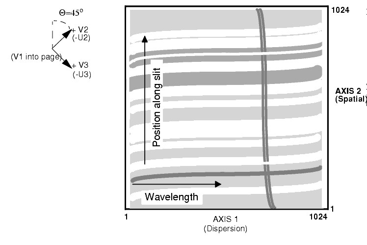
In MAMA ACCUM mode exposures, photons are accumulated into a 2048 x 2048, 16 bit per element oversampled array in the STIS data buffer memory as they are received. At the end of the exposure, the data can be left in the over-sampled (or highres) format, which is the default for scientific exposures, or they can be binned along axis1 and axis2 to produce a 1024 x 1024 native-format image. ACCUM is the mode of choice for all observations that do not require time resolution on minute or less scales. Dispersion runs along AXIS1 and the spatial dimension of the slit run along axis2. Figure 11.3 and Figure 11.4 illustrate the format and coordinate system for MAMA images, showing how first-order and echelle ACCUM mode spectrograms appear. prism images have dispersion along axis1. Note that for FUV-MAMA G140L and G140M the target is placed near AXIS2=392 to ensure that they will not fall on the shadow of the repeller wire (see Section 7.5). Thus there will be ~3 arcseconds less spatial sky coverage to decreasing AXIS2 and ~3 arcseconds more spatial sky coverage to increasing AXIS2 along the slit. Said another way, slit center will project ~3 arcseconds below the detector center along AXIS2 for G140L and G140M observations. Note also the effects of the monthly offsetting which applies to all MAMA modes (see Section 7.5). (Data taken prior to March 15, 1999 have the slit center offset above the detector center.)
The minimum MAMA ACCUM mode exposure time is 0.1 second and the maximum exposure time is 1.8 hours. The minimum time between identical MAMA ACCUM exposures is ~30 seconds, for exposures which are longer than 3 minutes, and it is 2.5 minutes for exposures which are shorter than 3 minutes. This difference arises because in the former case the buffer can be dumped to the HST recorder during the subsequent exposure (i.e., in parallel), but in the latter case there is insufficient time to dump the buffer during the subsequent exposure and the buffer must be dumped serially (i.e, using observing time).
For the MAMA medium-resolution, first-order modes and medium and high-resolution echelle modes (i.e., gratings G140M, G230M, E230M, E230H, E140M, and E140H), a correction for Doppler shifting of the photon energies due to HST spacecraft motion is applied as the photons are counted, prior to their addressing in STIS data-buffer memory. The leading and trailing pixels in the dispersion direction (axis1) for Doppler-corrected exposures therefore receive less effective integration time, since source photons at the corresponding wavelengths have been Doppler-shifted off the edge of the detector for some fraction of the total exposure time. This effect is strongest in the high-resolution echelle modes, where for a maximum HST spacecraft velocity of 7.5 km sec-1, the leading and trailing ~20 axis1 pixels will have reduced effective exposure times.
The MAMA detectors record scientific data in the so-called highres mode, producing 2048 x 2048 images of super resolution - one half the 1024 x1024 "native"-format pixel size defined by the anode readout itself. All scientific data are taken in this format by default. Below we explain in more detail the nature of highres data.
The MAMA detectors have 1024x1024 physical or so-called native-format pixels. However, each count is detected by multiple electrodes, so the charge distribution among the electrodes can be used to centroid the incident charge cloud to subpixel resolution. The gain of the highres 2048 x 2048 mode is a ~10-30% increase in resolution at the price of the increased fixed-pattern noise due to poorly characterized charge partition among the electrodes. The highres flat fields have much more structure than the 1024 x 1024 flats, with adjacent columns and rows differing by ~30% in an off/on pattern whose variability is appreciably higher than for 1024 x 1024 format images. This effect and the inherently lower signal-to-noise ratio in the full-resolution flat-field images (nominally ~20 to 1 per highres pixel) suggest that it may be difficult to routinely realize the benefit in resolution. However, we note that data taken in highres mode can always be binned to 1024 x 1024 on the ground in post-observation data processing, and since the extra overheads in highres mode are typically quite small, highres is the default data-taking mode for the MAMA. The pipeline bins the data to 1024 x 1024 format during calibration so that the pipeline-output calibrated images are native format (see the HST Data Handbook for more details).
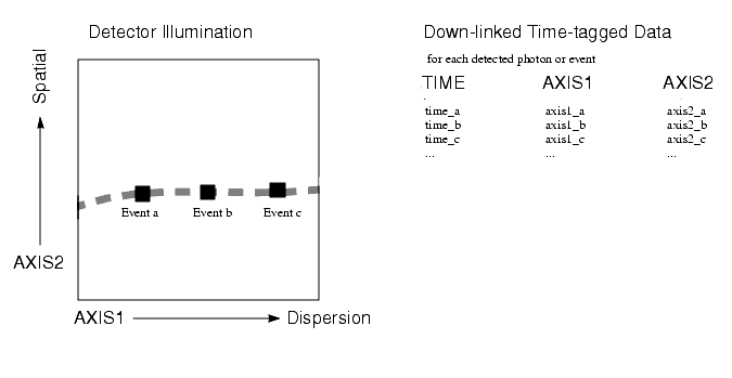
TIME-TAG mode is used for high-time-resolution spectroscopy and imaging in the ultraviolet. When used in TIME-TAG mode, the MAMA produces an event stream of axis1, axis2, and time data points, with a time resolution of 125 microseconds. The volume of data produced in TIME-TAG mode can be very large and the data therefore must be continuously transferred from the STIS internal buffer to the data recorders to sustain TIME-TAG exposures of any significant duration.
The axis orientation in TIME-TAG is the same as in ACCUM mode (see page Figure 11.3:). The spacecraft time (absolute zero point of the time) is routinely known to 10 millisecond accuracy. No Doppler correction is applied by the flight software for TIME-TAG mode, but the correction can be applied during the post-processing of the data. The recorded times are the spacecraft times, which can be converted to heliocentric times using the ephemeris of the Earth and the spacecraft. TIME-TAG mode is illustrated in Figure 11.5. Processing of TIME-TAG data by the STScI pipeline is described in Section 15.1.
In TIME-TAG mode, events detected on the anode wires are queued in a 4096-event FIFO prior to time assignment and subsequent storage in a STIS memory buffer. When the FIFO is less than half full, 4 events can be processed during each 125 microsecond tick of the STIS clock, corresponding to a maximum stable count rate of 32,000 counts/sec. Times are assigned shortly after detection, when the event is extracted from the FIFO. This is the desired operating state in TIME-TAG mode. Higher count rate situations (described below) should be avoided because they result in less accurate times, lost events, and buffer management problems.
For global count rates up to 50,000 counts/sec, the FIFO will gradually fill until more than 2048 events are queued. At this point 2048 events are processed in a tight loop requiring only 41 milliseconds, instead of the usual 64 milliseconds. Processing then reverts to the slower rate until the FIFO is again more than half full. In this mode, the times associated with each event have 125 microsecond resolution, but suffer from significantly larger systematic delays. Also, the observing sequence will be frequently interrupted to handle STIS buffer dumps (described below).
For count rates above 50,000 counts/sec, the FIFO will fill faster than events can be processed, even in fast mode. When the FIFO fills, all events in the FIFO are discarded and the empty FIFO begins filling with new events. In this mode event times are essentially uniform, providing essentially no information about source variability.
For TIME-TAG observations, STIS memory is divided into two 8 megabyte buffers, each of which can hold up to 2 x 10⁶ events. If the cadence between scheduled buffer dumps is at least 99 seconds, then one buffer can be actively recording new events, while previously recorded events in the other buffer are being dumped to an HST data recorder. Thus, events can be dumped to STIS memory without gaps only if the global count rate is below 20,000 counts/sec.
During Phase 2 proposal preparation, observers must specify in advance the time between dumps using the BUFFER-TIME parameter. The following constraints should be considered when selecting a BUFFER-TIME:
To prevent loss of data, BUFFER-TIME should be short enough that fewer than 2 x 10⁶ events are expected in the interval between dumps. If R is the expected count rate (predicted by the STIS Exposure Time Calculator, for example), then BUFFER-TIME should be smaller than 2 x 10⁶/R. A bit of margin protects against source variability or inaccurate count rate predictions. Be sure to include sky and detector backgrounds when estimating count rates.
On the other hand, the nominal STIS allocation on the HST data recorders allows at most 30 total buffer dumps in any one visit, and fewer is desirable. For the minimum continuously sustainable BUFFER-TIME of 99 seconds, this limit on dumps corresponds to a total exposure time of only 50 minutes. It is sometimes possible to schedule downlinks from the HST data recorders to the ground during a specific TIME-TAG visit. Thus, with a strong scientific justification, it may be possible to accommodate visits that require more than 30 dumps. Such requests should be justified quantitatively in the Phase 1 proposal.
Finally, BUFFER-TIME should be at least 99 seconds when more than 2 dumps are expected. Otherwise, the observing sequence will be interrupted whenever both buffers are in the process of being dumped. In such cases it is probably better to choose a BUFFER-TIME of 99 seconds. This guarantees that photons will be recorded whenever the active buffer has remaining space. If the active buffer fills in less than the selected BUFFER-TIME, additional photons will be discarded until the next dump begins. Reliable flux calibration is not possible in such cases.
In summary, BUFFER-TIME should be less than 2 x 10⁶/R, but longer than 1/30 the total exposure time and longer than 99 seconds. In some cases it will not be possible to satisfy all of these criteria, in which case multiple short ACCUM exposures should be considered as an alternative.
BUFFER-TIME. Tint refers to the total integration time (in sec) of all the exposures in the visit, and Texp refers to the integration time (in sec) of the particular exposure under consideration. 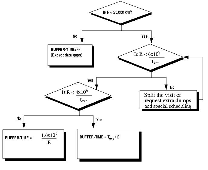
CR-SPLIT, i.e., if CR-SPLIT=3, there will be 3 x 45 seconds of overhead on the set of 3 exposures due to CCD setup and readout.
|
Space Telescope Science Institute http://www.stsci.edu Voice: (410) 338-1082 help@stsci.edu |